Introduction to the RSP Portal Aspect
Log in to the Portal Aspect by clicking on the “Portal” panel of the main landing page at data.lsst.cloud.
The Portal’s user interface
Across the top is a menu bar of interface options, but the DP0 data set is only accessed via the The Table Access Protocol (TAP) service reached via the “RSP TAP Search” button. Under TAP Searches there are four steps.
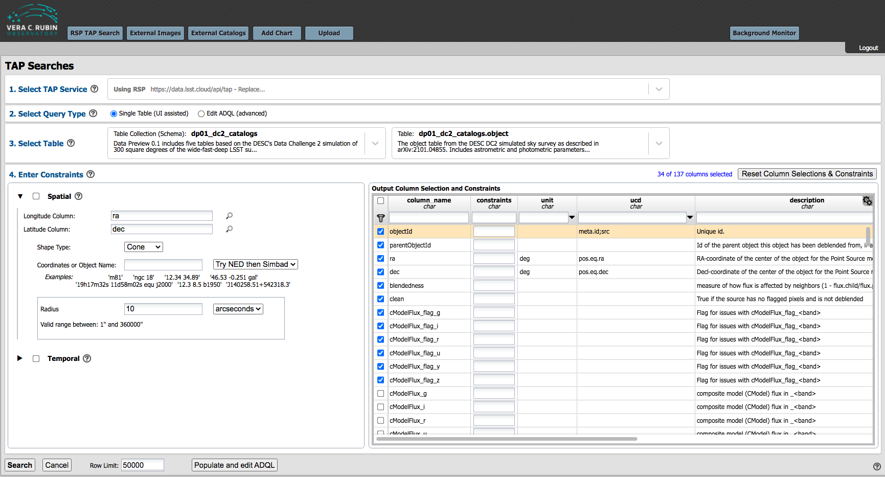
This is the default view upon entering the Portal Aspect.
Single Table Queries
1. TAP Service: Leave the default (https://data.lsst.cloud/api/tap) to access DP0 data.
2. Select Query Type: Select “Single Table (UI assisted)” to query via the single-table interface (default).
3. Select Table: Drop down menus of available tables. For DP0 data, choose the “Table Collection (Schema): dp01_dc2_catalogs”, and then choose the table to query (see the DP0.1 Data Products Definition Document (DPDD) for a reminder of what tables are available). The table view at lower-right will automatically update to match the selected table.
4. Enter Constraints: Only “Spatial” constraints apply for DP0.1.
The longitude and latitude columns will automatically update to be the correct column names for right ascension and declination for the selected table (usually ra and dec or coord_ra and coord_dec).
If a non-existent column name is entered the box will highlight red in indication of the error.
Choose the desired shape type for a spatial search, Cone or Polygon, and the appropriate instructions for the search terms will appear.
Keeping the search area to a minimum will keep processing times short and returned subsets small and manageable.
Note: The examples under the box for coordinates are object names as examples of the syntax and formatting only. Those examples are not guaranteed to be in the accessible data sets.
The central coordinates for DC2, in decimal degrees, are: 61.863 -35.790. (See Table 2 of The LSST DESC DC2 Simulated Sky Survey.)
Note: Although there are two options for “Constraints” (Spatial and Temporal), for DP0.1, all of the catalog data that is available through the Portal is from the coadded DC2 images, and does not contain time-domain information.
Table View: The table to the right of “Select Constraints” enables applying additional search constraints on the columns in the selected table. Use the checkboxes in the left-most column to select the columns to be returned by the query. Use the filter icon to only view selected columns. Many of the attributes of the table columns in the DC2 datasets are blank, but these are expected to be populated in the future Data Previews and Data Releases.
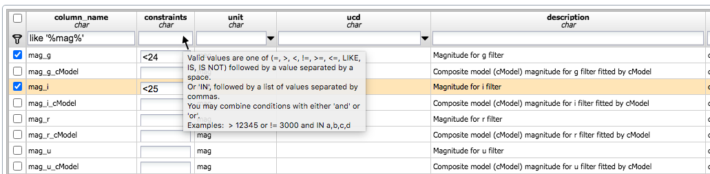
The table view offers additional query options.
Some tables have a lot of columns. Search for desired columns by entering terms in the boxes underneath “column_name” or “description”. Additional constraints on column data can be included in the query by specifying them under “constraints”. Mouse-over to view pop-up boxes with instructions.
Remove filters and reset the table view at any time using the “Remove” or “Reset” buttons above the upper-right corner of the table (not shown in image above).
If desired, convert table view queries to ADQL Queries using the “Populate and Edit ADQL” button at the bottom of the page. This can enable entering more complex constraints that cannot be expressed against individual columns.
Search: Press the search button at lower left when ready to execute.
The Row Limit may be changed to apply an upper bound to the number of rows returned. The Portal can work effectively with datasets with up to a million rows, or even more; however, in the present implementation of the RSP it is advisable to limit the number of columns requested for queries expected to return results on such a scale: SELECT * for 100,000+ rows can return datasets of unwieldy total size.
Note: Because of the implementation of the Rubin Observatory Qserv database, it is not recommended to use the row limit alone in order to get a “sampling” of data. Queries with only a row limit can run for much longer than one might intuitively expect; applying a spatial constrain is likely to return a result more quickly.
The example in the image below queries the dp01_dc2_catalogs.object table using a cone search centered on 61.863 -35.790 in decimal degrees (the approximate center of the DC2 region) with a 200 arcsec radius.
The search will return data in columns ra, dec, mag_g, and mag_i for all objects with mag_g and mag_i brighter than 24th magnitude.
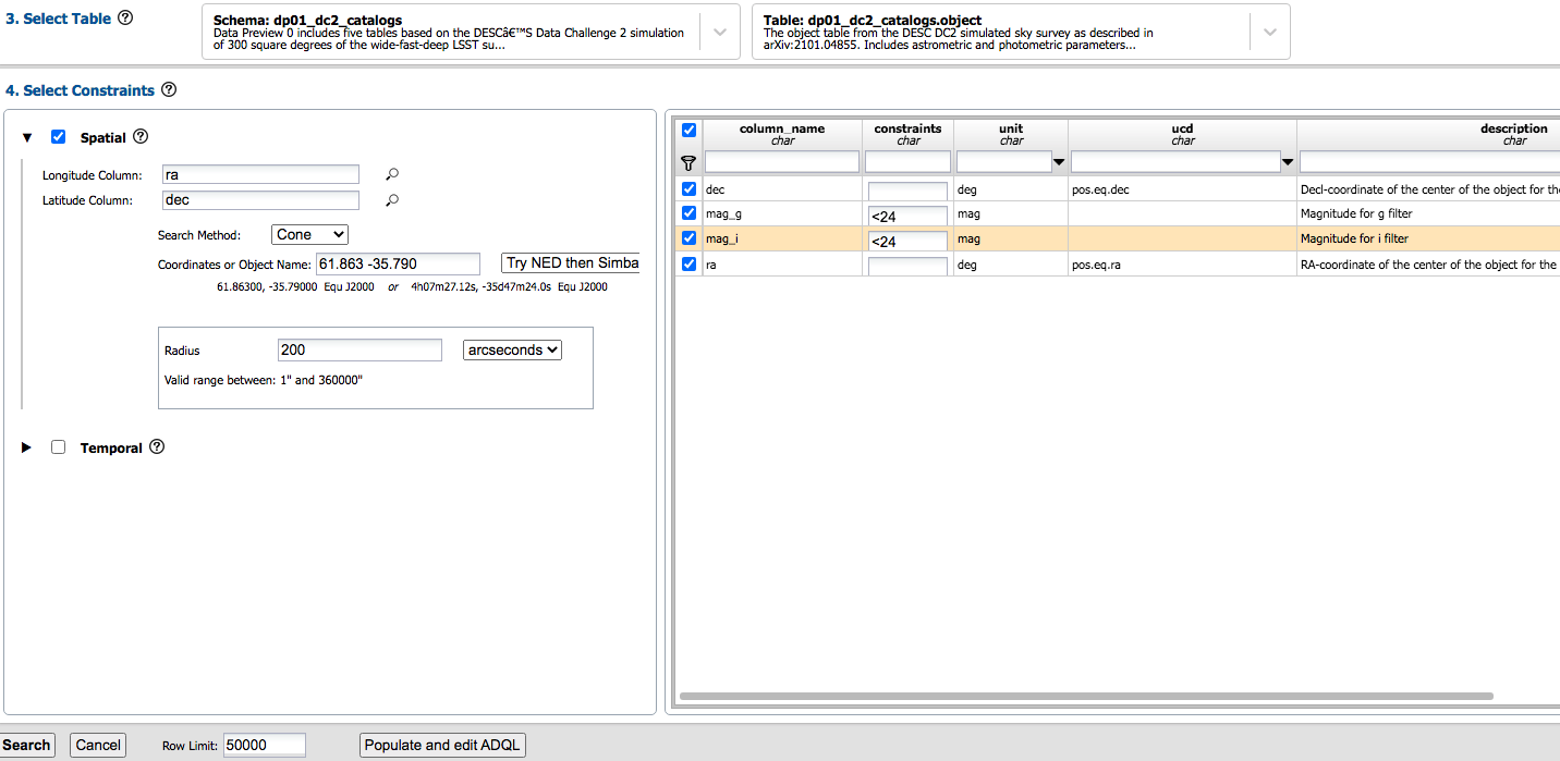
An example query of the DC2 Object catalog.
This will show while the search is executing.
Results View: The search results will populate the results view, as shown in the next figure.
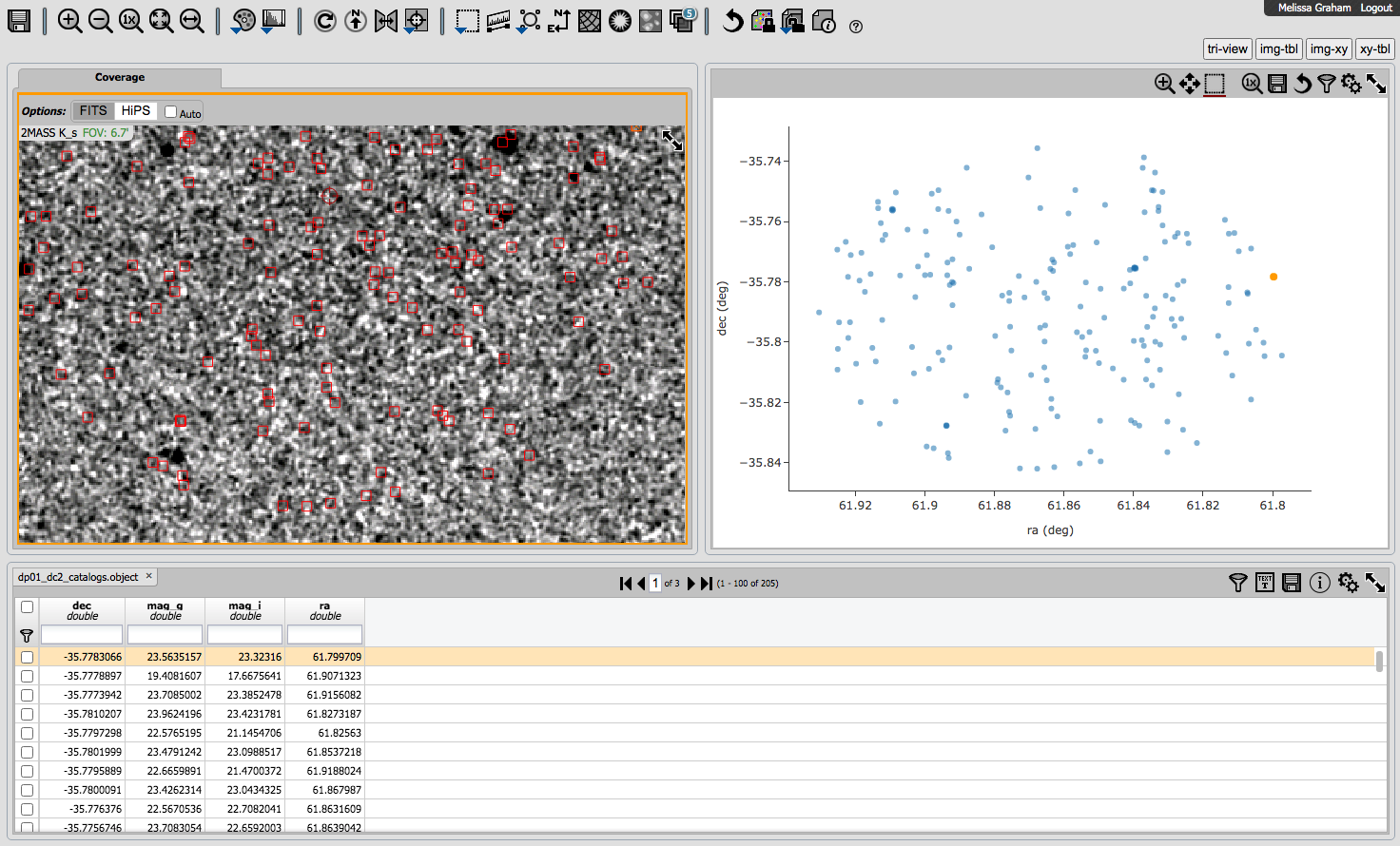
The default view of the search results.
Across the top of the results view are many icons that control the display settings; hover over the icons and a statement about their functionality will appear at upper-right. Also at upper right, under the user name, are the options “tri-view”, “img-tbl”, “img-xy”, and “xy-tbl”. These control how the results view is partitioned, and the default is “tri-view”. In the “tri-view”, at top-left is a sky image with the search results overplotted, but note that this is not a simulated DC2 image, but a 2MASS image. Select “HiPS” and a “Change HiPS” button will appear with options for sky images to use, but none of the options are relevant for the DC2 simulated sky data. Thus for DP0, the “xy-tbl” is the most relevant view for results.
To manipulate the plotted data, select the double gear “settings” icon above the x-y plot and a pop-up window will open (see the next figure). Select other columns to use, change the symbol type and color, and so forth, and click “Apply”.
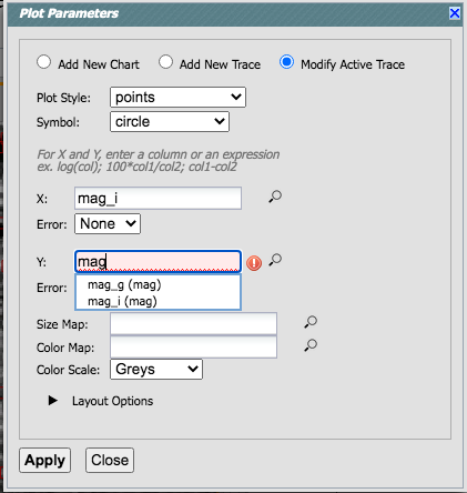
The plot settings pop-up window.
Additional cuts can be applied to the plotted data using the table query boxes, such as in the next image where a limit of mag_g brighter than 22 mag is used.
Note that corresponding plot point for the selected row in the table is differently colored, and that hovering the mouse over the plotted data will show the x- and yvalues in a pop-up window.
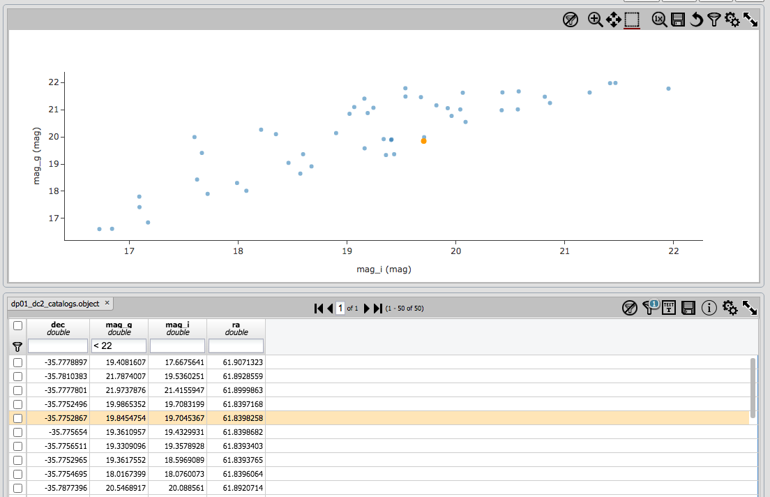
An updated results view in which the xy plot uses the magnitude columns.
See also Portal aspect demonstrations for additional demonstrations of how to use the Portal’s Single Table Query.
ADQL Queries
1. TAP Service: Leave the default (https://data.lsst.cloud/api/tap) to access DP0 data.
2. Select Query Type: Select “ADQL” to query via the ADQL interface. ADQL is the Astronomical Data Query Language. The language is used by the IVOA to represent astronomy queries posted to Virtual Observatory (VO) services, such as the Rubin LSST TAP service. ADQL is based on the Structured Query Language (SQL).
3. Advanced ADQL: When ADQL is selected as the query type, the interface in step 3 changes to provide a free-form block into which ADQL queries can be entered directly. The query executed in the Single Table Queries example above can be expressed in ADQL as follows:
SELECT ra, dec, mag_g, mag_i
FROM dp01_dc2_catalogs.object
WHERE CONTAINS(
POINT('ICRS', ra, dec),
CIRCLE('ICRS', 61.863, -35.79, 0.05555555555555555))=1
AND (mag_g <24 AND mag_i <24)
Type the above query into the ADQL Query block and click on the “Search” button in the bottom-left corner to execute. You should set the row limit to be a small number, such as 10, when first testing queries. The search results will populate the same Results View, as shown above using the Single Table Query interface. A total of 205 records should be returned, which you can interact with in the same manner as outlined in Single Table Queries.
Joining with another table
It is often desirable to access data stored in more than just one table.
We do this using a JOIN clause to combine rows from two or more tables.
Here, using the same query as above, we will join the data in the object table with the data in the truth table to compare the results of the processing with the input truth information.
The two tables are joined by matching the objectId across two catalogs.
SELECT obj.ra as ora, obj.dec as odec,
truth.ra as tra, truth.dec as tdec,
obj.mag_g as g, obj.mag_i as i, obj.mag_r as r,
truth.mag_r as tmr, truth.is_good_match
FROM dp01_dc2_catalogs.object as obj
JOIN dp01_dc2_catalogs.truth_match as truth
ON truth.match_objectId = obj.objectId
WHERE CONTAINS(
POINT('ICRS', obj.ra, obj.dec),
CIRCLE('ICRS', 61.863, -35.79, 0.05555555555555555))=1
AND (obj.mag_g <24 AND obj.mag_i <24)
AND truth.is_good_match = 1
This query also includes some additional quality filtering on the match.
In the truth_match table, is_good_match is true (or 1) if an object-truth matching pair satisfies all matching criteria, or it is false``(or ``0) otherwise.
is_good_match for an object is defined as, separations <1 arcsec and magnitude differences <1 mag.
This reduces the number of results returned from 205 to 191.
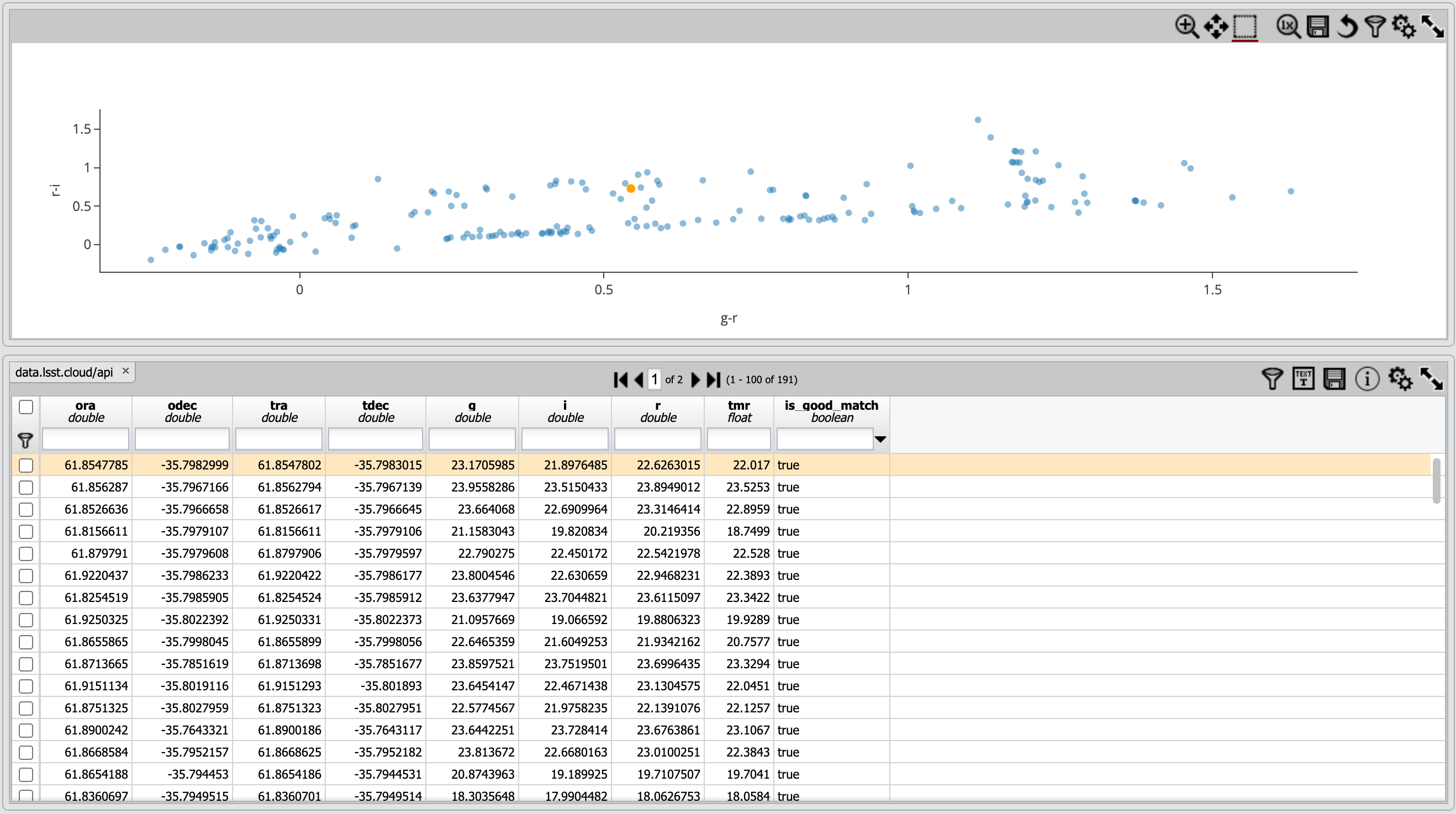
The results of a JOIN.
Note that is_good_match is of type boolean whereas in the ADQL query above we selected good matches by filtering on truth.is_good_match = 1 . With ADQL, the “=0” (false) or “=1” (true) syntax for booleans should be used.
Query the TAP service schema Information about the LSST TAP schema can also be obtained via ADQL queries. The following query gets the names of all the available DP0.1 tables.
SELECT *
FROM tap_schema.tables
WHERE tap_schema.tables.table_name like 'dp01%'
To get the detailed list of columns available in the object table, their associated units and descriptions:
SELECT tap_schema.columns.column_name, tap_schema.columns.unit,
tap_schema.columns.description
FROM tap_schema.columns
WHERE tap_schema.columns.table_name = 'dp01_dc2_catalogs.object'
This produces a subset of the data shown in the lower-right pane of the Portal’s Single Table query screen, described above.
See also Portal aspect demonstrations for additional demonstrations of how to use the Portal’s ADQL functionality.